39 display data labels excel
Chart: Display alternative values as Data Labels or Data Callouts Joined. Aug 11, 2017. Messages. 1. Aug 11, 2017. #1. Below is my excel chart. I would like to add a "data labels" or "data callouts". As you can see the line is displaying the data from Actual X and Y, but I want to display the DEV values on this line. Excel charts: how to move data labels to legend - Microsoft Tech Community @Matt_Fischer-Daly . You can't do that, but you can show a data table below the chart instead of data labels: Click anywhere on the chart. On the Design tab of the ribbon (under Chart Tools), in the Chart Layouts group, click Add Chart Element > Data Table > With Legend Keys (or No Legend Keys if you prefer)
Office: Display Data Labels in a Pie Chart 3. In the Chart window, choose the Pie chart option from the list on the left. Next, choose the type of pie chart you want on the right side. 4. Once the chart is inserted into the document, you will notice that there are no data labels. To fix this problem, select the chart, click the plus button near the chart's bounding box on the right ...
Display data labels excel
How to Use Cell Values for Excel Chart Labels Select the chart, choose the "Chart Elements" option, click the "Data Labels" arrow, and then "More Options.". Uncheck the "Value" box and check the "Value From Cells" box. Select cells C2:C6 to use for the data label range and then click the "OK" button. The values from these cells are now used for the chart data labels. How to Add Labels to Scatterplot Points in Excel - Statology Step 3: Add Labels to Points Next, click anywhere on the chart until a green plus (+) sign appears in the top right corner. Then click Data Labels, then click More Options… In the Format Data Labels window that appears on the right of the screen, uncheck the box next to Y Value and check the box next to Value From Cells. How to Create Labels in Word from an Excel Spreadsheet Select the Mailings tab at the top and then select Update Labels. All labels in your document should now say <>. 5. Create Labels From Excel in a Word Document Word now has all the data it needs to generate your labels. You will now finish the process and Word will display the actual data for each label:
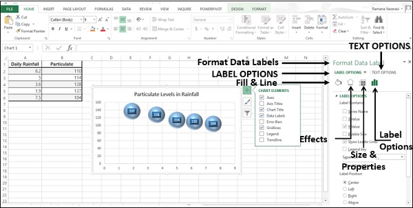
Display data labels excel. How to add data labels from different column in an Excel chart? Right click the data series in the chart, and select Add Data Labels > Add Data Labels from the context menu to add data labels. 2. Click any data label to select all data labels, and then click the specified data label to select it only in the chart. 3. How to show data label in "percentage" instead of - Microsoft Community Select Format Data Labels Select Number in the left column Select Percentage in the popup options In the Format code field set the number of decimal places required and click Add. (Or if the table data in in percentage format then you can select Link to source.) Click OK Regards, OssieMac Report abuse 8 people found this reply helpful · Change the format of data labels in a chart To get there, after adding your data labels, select the data label to format, and then click Chart Elements > Data Labels > More Options. To go to the appropriate area, click one of the four icons ( Fill & Line, Effects, Size & Properties ( Layout & Properties in Outlook or Word), or Label Options) shown here. Data labels not displayed correctly - Excel Help Forum The data label is a date value that selects values from the date column. The Primary axis is categorized based on 2 values. The secondary axis is Month. The data labels are displayed accurately as per the month except the 3 labels. The first series is the difference between F and E.The second series is the difference between the J and K column.
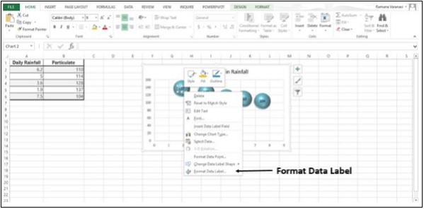
How to Add Data Labels to an Excel 2010 Chart - dummies Use the following steps to add data labels to series in a chart: Click anywhere on the chart that you want to modify. On the Chart Tools Layout tab, click the Data Labels button in the Labels group. A menu of data label placement options appears: None: The default choice; it means you don't want to display data labels. Center to position the ... Add data labels and callouts to charts in Excel 365 - EasyTweaks.com Step #3: Format the data labels. Excel also gives you the option of formatting the data labels to suit your desired look if you don't like the default. To make changes to the data labels, right-click within the chart and select the "Format Labels" option. How to use data labels in a chart - YouTube Excel charts have a flexible system to display values called "data labels". Data labels are a classic example a "simple" Excel feature with a huge range of o... How to add data labels in excel to graph or chart (Step-by-Step) 1. Select a data series or a graph. After picking the series, click the data point you want to label. 2. Click Add Chart Element Chart Elements button > Data Labels in the upper right corner, close to the chart. 3. Click the arrow and select an option to modify the location. 4.
Can you display data labels on a trend line? - MrExcel Message Board Hi I have plotted some sales figures on a line chart (Jan-Aug), and added a linear trend line to view the trend to the end of the year. I have not used the 'forecast forward 4 periods' feature to do this, instead I have just selected an additional 4 blank rows below the 'august' line - which extends the x axis, and therefore extends the trend line. Custom Chart Data Labels In Excel With Formulas Follow the steps below to create the custom data labels. Select the chart label you want to change. In the formula-bar hit = (equals), select the cell reference containing your chart label's data. In this case, the first label is in cell E2. Finally, repeat for all your chart laebls. Quick Tip: Excel 2013 offers flexible data labels | TechRepublic right-click and choose Insert Data Label Field. In the next dialog, select [Cell] Choose Cell. When Excel displays the source dialog, click the cell that contains the MIN () function, and click OK.... Excel tutorial: How to use data labels Generally, the easiest way to show data labels to use the chart elements menu. When you check the box, you'll see data labels appear in the chart. If you have more than one data series, you can select a series first, then turn on data labels for that series only. You can even select a single bar, and show just one data label.
Advanced Excel - более богатые метки данных - CoderLessons.com
How to Add Data Labels in Excel - Excelchat | Excelchat In Excel 2013 and the later versions we need to do the followings; Click anywhere in the chart area to display the Chart Elements button Figure 5. Chart Elements Button Click the Chart Elements button > Select the Data Labels, then click the Arrow to choose the data labels position. Figure 6. How to Add Data Labels in Excel 2013 Figure 7.
Excel Dashboards - Краткое руководство - CoderLessons.com
Adding rich data labels to charts in Excel 2013 | Microsoft 365 Blog Putting a data label into a shape can add another type of visual emphasis. To add a data label in a shape, select the data point of interest, then right-click it to pull up the context menu. Click Add Data Label, then click Add Data Callout . The result is that your data label will appear in a graphical callout.
Custom data labels in a chart | Get Digital Help - Microsoft Excel resource
to display top 5 data labels on graph [SOLVED] - Excel Help Forum Re: to display top 5 data labels on graph. Also, I noticed your sum column ("total") is returning errors. I don't see why you would want to do this, and in fact I'm not even sure why excel wanted to do this to begin with. if you run C3+D3 when those cells are empty, excel should return 0. So I got rid of the error, and that way, you can use the ...

Line Chart in Excel - Easy Excel Tutorial
Add or remove data labels in a chart - support.microsoft.com Right-click the data series or data label to display more data for, and then click Format Data Labels. Click Label Options and under Label Contains, select the Values From Cells checkbox. When the Data Label Range dialog box appears, go back to the spreadsheet and select the range for which you want the cell values to display as data labels.
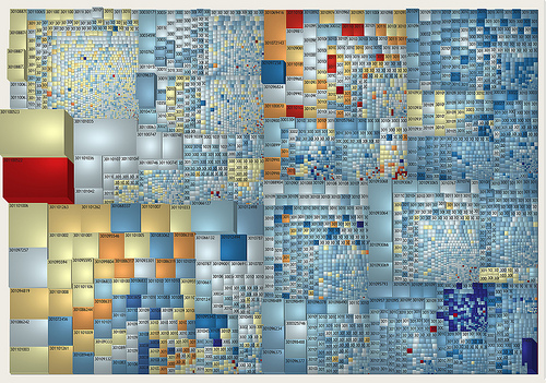
TreeMap
Excel Charts: Creating Custom Data Labels - YouTube In this video I'll show you how to add data labels to a chart in Excel and then change the range that the data labels are linked to. This video covers both W...
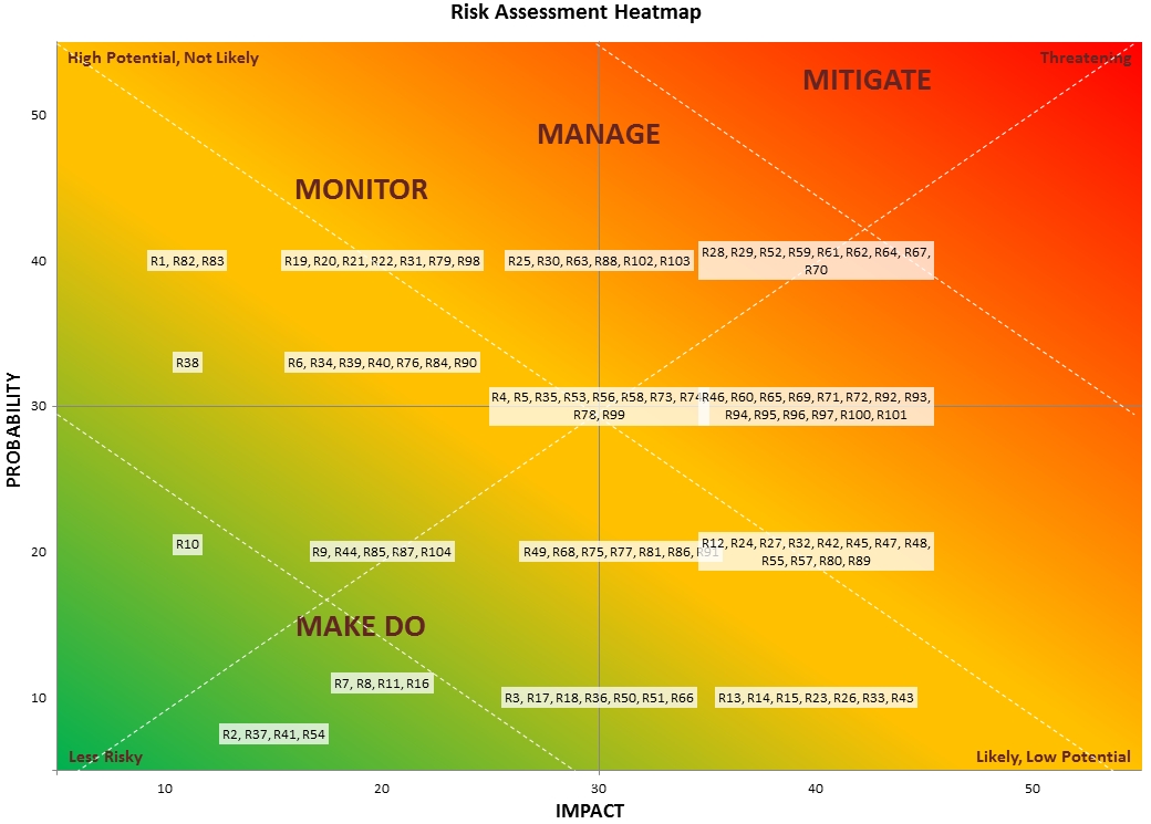
How to Create a Risk Heatmap in Excel - Part 2 - Risk Management Guru
How to add or move data labels in Excel chart? - ExtendOffice 2. Then click the Chart Elements, and check Data Labels, then you can click the arrow to choose an option about the data labels in the sub menu. See screenshot: In Excel 2010 or 2007. 1. click on the chart to show the Layout tab in the Chart Tools group. See screenshot: 2. Then click Data Labels, and select one type of data labels as you need ...

Column vs Bar Charts in Excel | A4 Accounting
Display every "n" th data label in graphs - Microsoft Community With this tool you can assign a range of cells to be the labels for chart series, instead of the Excel defaults. Using a formula, you can have a text show up in every nth cell and then use that range with the XY Chart Labeler to display as the series label. If the full chart labels are in column A, starting in cell A1, then you can use this ...
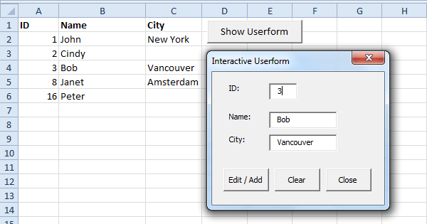
Excel VBA Interactive Userform - Easy Excel Macros
Custom Data Labels with Colors and Symbols in Excel Charts - [How To] Step 4: Select the data in column C and hit Ctrl+1 to invoke format cell dialogue box. From left click custom and have your cursor in the type field and follow these steps: Press and Hold ALT key on the keyboard and on the Numpad hit 3 and 0 keys. Let go the ALT key and you will see that upward arrow is inserted.
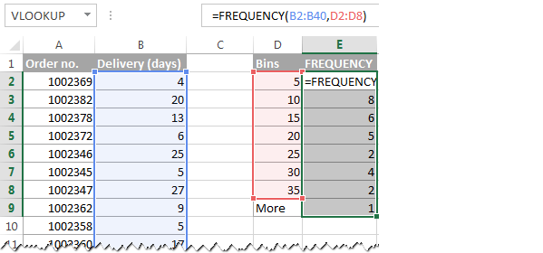
How to make a histogram in Excel 2019, 2016, 2013 and 2010
10 spiffy new ways to show data with Excel | Computerworld 10 spiffy new ways to show data with Excel ... Right-click the X-axis labels and click Format Axis. In the Axis Options pane, click the Number item and, in Category, select Date from the drop-down ...
Post a Comment for "39 display data labels excel"