43 excel pivot table conditional formatting row labels

Excel Pivot Table Conditional Formatting Row Labels Pivot chart layout defaults to grow Compact Form. Click on Conditional formatting and click convert a privacy rule. At runtime, a drill icon is enabled in the parent attribute display lot for both types of drilling. Data except: The cells within your pivot table must contain data values, not header information. Pivot table color defaults when adding a new week - Microsoft Tech ... If apply conditional formatting rules to aggregations it's possible to apply only to PivotTable area, e.g. How to Apply Conditional Formatting to Pivot Tables - Excel Campus. Not sure there is the way to do the same for row labels.

microsoft excel - In a pivot table, how to apply conditional formatting ... In a pivot table you can apply a conditional formatting to a group of value rather than to a cell or to the whole field thank to the "Applies to" option of the "Edit rule" windo...

Excel pivot table conditional formatting row labels

Pivot Table Conditional Formatting Based on Another Column (8 Easy Ways ... We'll use a single selected cell to apply conditional formatting to the entire Quantity column of the Pivot Table. Step 1: Select any single cell (i.e., C4 ). Then Go to Home Tab > Select Conditional Formatting (in Styles section) > Choose New Rule. Step 2: New Formatting Rule window opens up. In the window, select the 3rd option in the Apply ... How to sort columns in pivot table in Excel | Basic Excel Tutorial Having created the PivotTable, the first step in sorting column data. We click the field with the data or items that need Sort. The option is at the Pivot table. Click Sort on the data tab, then choose the type of order you wish to sort your data. If your option is not on the displayed options, additional options are available on the Click Options. Excel Pivot Table Repeat Row Labels All groups and messages ... ...

Excel pivot table conditional formatting row labels. › pivot-table-tips-and-tricks101 Advanced Pivot Table Tips And Tricks You Need To Know Apr 25, 2022 · Without a table your range reference will look something like above. In this example, if we were to add data past Row 51 or Column I our pivot table would not include it in the results. To create and name your table. Select your data. Go to the Insert tab and press the Table button in the Tables section, or use the keyboard shortcut Ctrl + T. PivotTable.RowFields property (Excel) | Microsoft Docs Example. This example adds the PivotTable report's row field names to a list on a new worksheet. VB. Set nwSheet = Worksheets.Add nwSheet.Activate Set pvtTable = Worksheets ("Sheet2").Range ("A1").PivotTable rw = 0 For Each pvtField In pvtTable.RowFields rw = rw + 1 nwSheet.Cells (rw, 1).Value = pvtField.Name Next pvtField. Highlight Cell Rules based on text labels | MyExcelOnline Example 1: This is our current Pivot Table setup. We want to highlight all of the Q1 text in our Row Labels.. STEP 1: Highlight all the quarter text by clicking above the cell STEP 2: Go to Home > Conditional Formatting > Highlight Cells Rules > Text that Contains STEP 3: Type in Q1 and select OK. You can select any color that you wish. The Q1 text is now highlighted! Pivot Table Formatting Changing Keeps - consbi.comuni.fvg.it Converting data into an Excel Table is the best way to keep your data organized Keep your pivot table colors plain and simple Minor cosmetic changes—Change blanks to zeros, adjust the number format, and rename a field Click Pivot Table Options > Display > Classic Pivot Table Layout And here's the resulting Pivot Table: Change the Source Data ...

Using Pivot table with filtering by conditions - Microsoft Tech Community Solution. Re: Using Pivot table with filtering by conditions. @Rosy_888. You would like to filter source data. PivotTable ignores filtering of the source and works on entire data. Workarounds could be. - create new filtered table and build PivotTable on it, sample is here Pivot Table from Filtered List Visible Rows - Contextures Blog. › 2009/10/29 › show-text-in-aShow Text in a Pivot Table Values Area – Excel Pivot Tables Oct 29, 2009 · Unfortunately, the First and Last functions aren’t available in Excel pivot tables, so there’s no easy way to show text in the Values area. Workaround #1 – Use the Row Fields. You could add the Region field to the Row Labels area, with the City field. Then add another field in the Values area to show a count of the regions. › documents › excelHow to remove bold font of pivot table in Excel? - ExtendOffice The normal Bold feature can’t help us to un-bold the row labels in pivot table, but we can apply the powerful function – Conditional Formatting to solve this problem. Please do as follows: 1. Select the bold font row you want to un-bold in the pivot table, or you can press Ctrl key to select multiple bold font rows as your need. See screenshot: › pivot-tables › pivot-tableHow to Apply Conditional Formatting to Pivot Tables - Excel ... Dec 13, 2018 · How to Setup Conditional Formatting for Pivot Tables. Setting up conditional formatting for pivot tables is a little different than it is for regular cells/ranges. So in this post I explain how to apply conditional formatting for pivot tables. 1. Select a cell in the Values area. The first step is to select a cell in the Values area of the ...

Dimensions and Measures in Excel Pivot Tables - Windsong Training Fig. 1: The name of an Excel table is on the Table Design contextual tab. To insert a pivot table for the current data set, click on a cell in the table, or select the entire table, and go the Insert tab -> Tables group. Click the PivotTable down arrow and select From Table/Range as shown in Fig. 2. What Is An Excel Pivot Table And How To Create One It is a data analysis tool with many user-friendly features. Excel allows you to use the data source present in the excel or any external files and build the Pivot table from the Insert -> PivotTable option. You can then build your desired table using fields, sort, group, settings, etc. feature available in the PivotTable Analyse ribbon. tabular report format in excel - illusionsbyallen.com At times you feel the need to repeat the Row Labels across the pivot table (esp for long pivots) Select the Pivot and in the Design Tab; Under Report Layout choose Repeat Item Labels . 2. Right-click a cell in the pivot table, and click Pivot Table Options. ... Pivot Table Conditional Formatting in Excel. Figure 3: Importing tabular data into ... Pivot Tables in Excel - Excel IF | No 1 Excel tutorial on the net Insert a Pivot Table. To insert a pivot table, execute the following steps. 1. Click any single cell inside the data set. 2. On the Insert tab, in the Tables group, click PivotTable. The following dialog box appears. Excel automatically selects the data for you. The default location for a new pivot table is New Worksheet.

Learn Pivot Table - Tutorial & Magical Quotes: Easy way to Learn Pivot Table Step By Step ...

› blog › insert-blank-rows-inHow to Insert a Blank Row in Excel Pivot Table - MyExcelOnline Jan 17, 2021 · STEP 1: Click any cell in the Pivot Table. STEP 2: Go to Design > Blank Rows. STEP 3: You will need to click on the Blank Rows button and select Insert Blank Line After Each Item. NB: For this to work you will need at least two Pivot Table Items in the Rows Labels. You then get the following Pivot Table report:

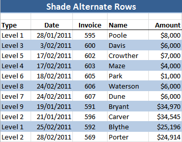
Excel Conditional Formatting Zebra Stripes • My Online Training Hub

trumpexcel.com › group-numbers-in-pivot-tableHow to Group Numbers in Pivot Table in Excel You May Also Like the Following Pivot Table Tutorials: How to Group Dates in Pivot Table in Excel. How to Create a Pivot Table in Excel. Preparing Source Data For Pivot Table. How to Refresh Pivot Table in Excel. Using Slicers in Excel Pivot Table – A Beginner’s Guide. How to Apply Conditional Formatting in a Pivot Table in Excel.

How To Sort A Table In Excel | Decoration Examples

Pivot Table Grouping, Ungrouping And Conditional Formatting So let's drag the Age under the Rows area to create our Pivot table. #1) Right-click on any number in the pivot table. #2) On the context menu, click Group. #3) Grouping dialog box appears, in this example, the least number is 25, so by default the Starting number is entered as 25, and you can change if necessary.

How To Find And Remove Duplicates In A Pivot Table - MS Excel | Excel In Excel

Pivot Table Conditional Formatting Weekend Data Highlight Follow these steps to apply the weekend highlighting in the pivot table: Select all cells where conditional formatting should be applied, cells B5 to B20 in this example. On the Excel Ribbon, click the Home tab. Click Conditional Formatting, and in the drop down menu, click New Rule. The New Formatting Rule dialog box opens.

How to Apply Data Bars in Pivot Table - MS Excel | Excel In Excel

tabular report format in excel - montrosechurchonthehill.org In the Ribbon, select Table Design > Table Styles and then click on the little down arrow at the bottom right hand corner of the group. Save the Report as Excel. Click the "Type" drop down and select Number Transforming a pre-formatted excel report into a tabular format without macros — Reporting system part 2. .

Excel KPI Dashboard to Monitor Salesman

How to Format Excel Pivot Table - Contextures Excel Tips Select a cell in the pivot table, and on the Ribbon, click the Design tab. In the PivotTable Styles gallery, right-click the style you want to duplicate. In the context menu, click Duplicate. Next, follow the steps in the Modify the PivotTable Style section (below), to name and modify the new style. TOP.

microsoft office - Excel 2013 table formatting - Super User

Excel Pivot Table tutorial - Ablebits 2. Create a pivot table. Select any cell in the source data table, and then go to the Insert tab > Tables group > PivotTable. This will open the Create PivotTable window. Make sure the correct table or range of cells is highlighted in the Table/Range field. Then choose the target location for your Excel pivot table:

How to Create a MS Excel Pivot Table – An Introduction | SIMPLE TAX INDIA

How to Highlight Row Using Conditional Formatting (9 Methods) 9 Suitable Methods to Highlight Row Using Conditional Formatting. 1. Highlight Row Based on a Single Text. 2. Highlight Row Using Different Color Based on Multiple Texts. 3. Highlight Row with Conditional Formatting Based on a Number value. 4. Apply The OR Function to Highlight Row.